Introduction

Maybe you’ve heard somewhere that physics is heavily math based. And yes, while that is true, a basic understanding of simple mathematics is sufficient to learn physics conceptually. It’s simply that most places don’t teach good conceptual physics anymore.

The Vector

The first thing we must recognize when we learn physics is the vector. The vector looks like an arrow, but it doesn’t tell you where to go! There are two important things to recognize about a vector: the length (we call "magnitude") and its direction. Remember those two things, and you will be pretty much set for the rest of physics.As you probably realize, all physics is based on math, which is why we start with a lesson in math. Scalar quantities, which are the quantities most are familiar with from math courses, are prevalent in physics. These have a magnitude, which is the value of the quantity.

Scalars are simply just the numbers you see and use in your math course. For example, $3$, is a scalar. However, in the real world (which is the realm physics operates in), we realize that something called "direction" exists. This is why we define vector quantities. They are quantities that have both magnitude and direction. Graphically, the direction is the direction in which the arrow points, and the magnitude is the length of the arrow.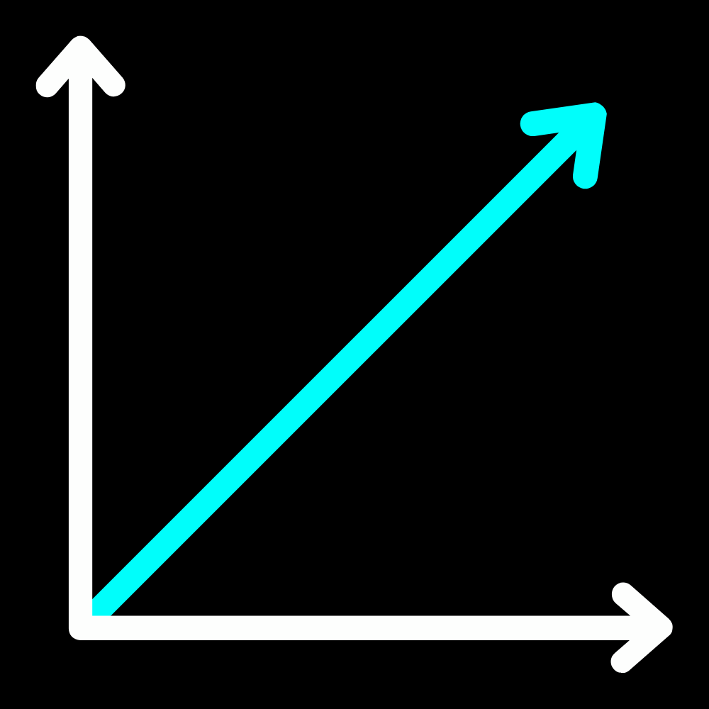

It is important to note that the position of the vector on the coordinate grid does NOT actually matter, so we can move them around the grid to make things more convenient. As long as we maintain the same direction and magnitude, we can move the vector around however we like.

Notation

A vector is defined and named by a single letter. A vector is typically seen with an arrowhead on top, like shown:  $\vec{a}$
In typed text, it is typically represented with a bold letter like this:  $\vectorbold{a}$

We will be using the arrowhead notation since it is a bit more noticeable in the midst of the oceans of text we're pouring on you. However, we're putting both notations out there just so you know for your reference. It is important to note that the position of the vector on the coordinate grid does NOT actually matter, so we can move them around the grid to make things more convenient. As long as we maintain the direction and magnitude, we are all good.

Notation

On paper, vectors are named with a single letter, much like variables. While scalars are defined just by a single letter (like $a$), a vector is defined by a letter with an arrowhead across its top, like so:  $\vec{a}$

In typed text and many textbooks out there, it is typically represented with a bold letter like this:  $\vectorbold{a}$

We will be using the arrowhead notation since it is a bit more noticeable in the midst of the oceans of text we're pouring on you. However, we're putting both notations out there just so you know for your reference.

Vector Addition

Now you're probably thinking, can you perform basic operations on vectors? Well, you can! However, it isn't as simple as $1+1=2$. There are times though, if two vectors point in the SAME direction, then you can add them like you would with normal numbers. (see below.)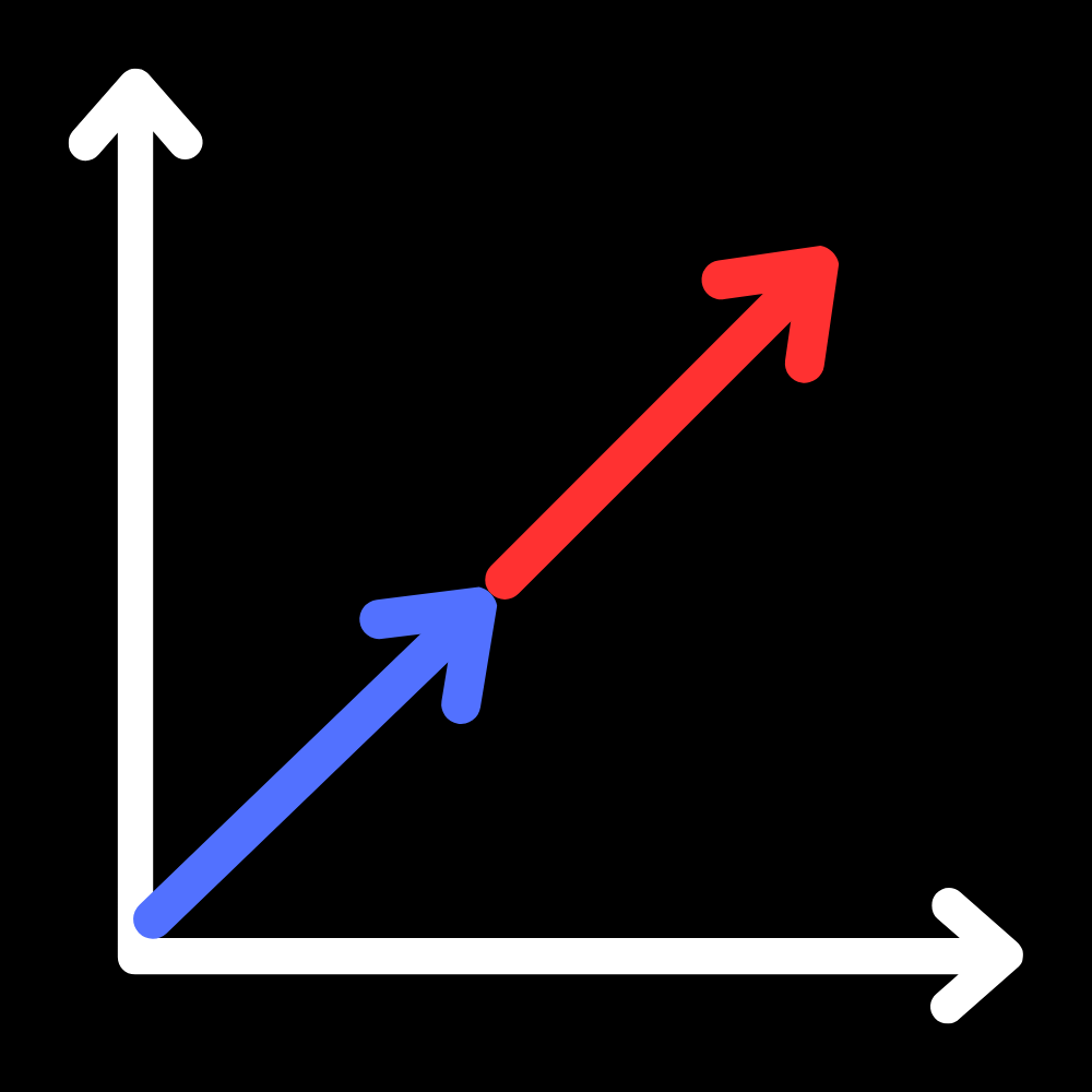

Other than that, there are two primary methods to adding vectors, one being algebraically and the other being graphically. We will focus on the latter since we aren't doing the algebra-based version.

Now, graphically, there are two main methods. Remember when we said the position of the vector doesn't matter? This will come in handy here. The tip to tail method involves placing the “tail” (the end without an arrow) of one vector to the “tip” (the arrowhead) of another, and drawing the resultant (final) vector from the starting point to the ending point. Perhaps a diagram will be more enlightening...

Vector Addition

While scalar quantities can be added linearly, vector quantities require a bit more work to manipulate. There are times, however, when you can add vectors linearly. That is when they are pointing in the same direction, as the diagram shows:

Besides that, you can either add them graphically or algebraically.

Graphical Methods

Graphically, there are two main methods, tip-to-tail and parallelogram. We will utilize the ability to reposition vectors anywhere on the coordinate grid for this. The tip to tail method involves placing the “tail” (the end without an arrow) of one vector to the “tip” (the arrowhead) of another, and drawing the resultant vector from the tail of the latter to the tip of the former. Perhaps a diagram will be more enlightening...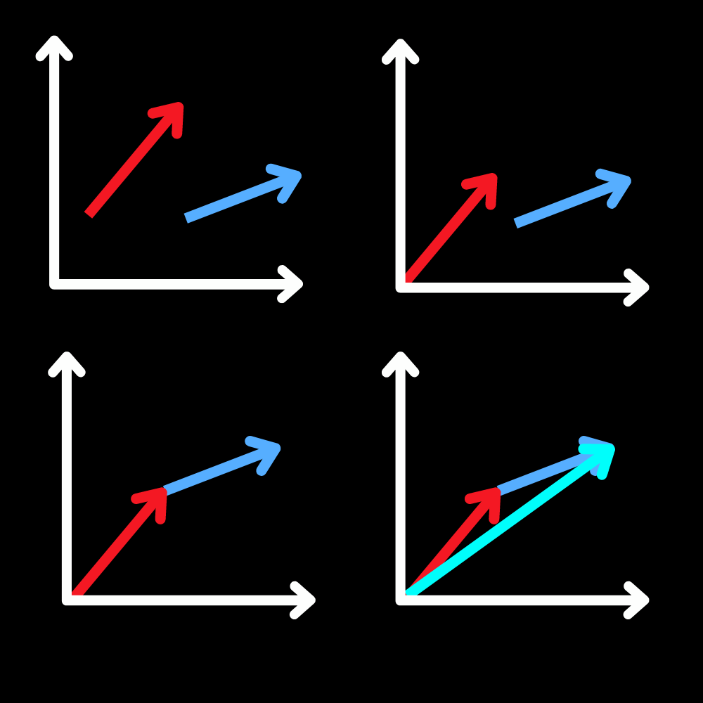

In the parallelogram method, both vectors are placed at the origin, and a parallelogram is drawn with the two vectors as adjacent sides. The resultant vector runs from the origin to the opposite vertex of the parallelogram. It is very similar to the tip-to-tail method, as you can see via the dashed lines.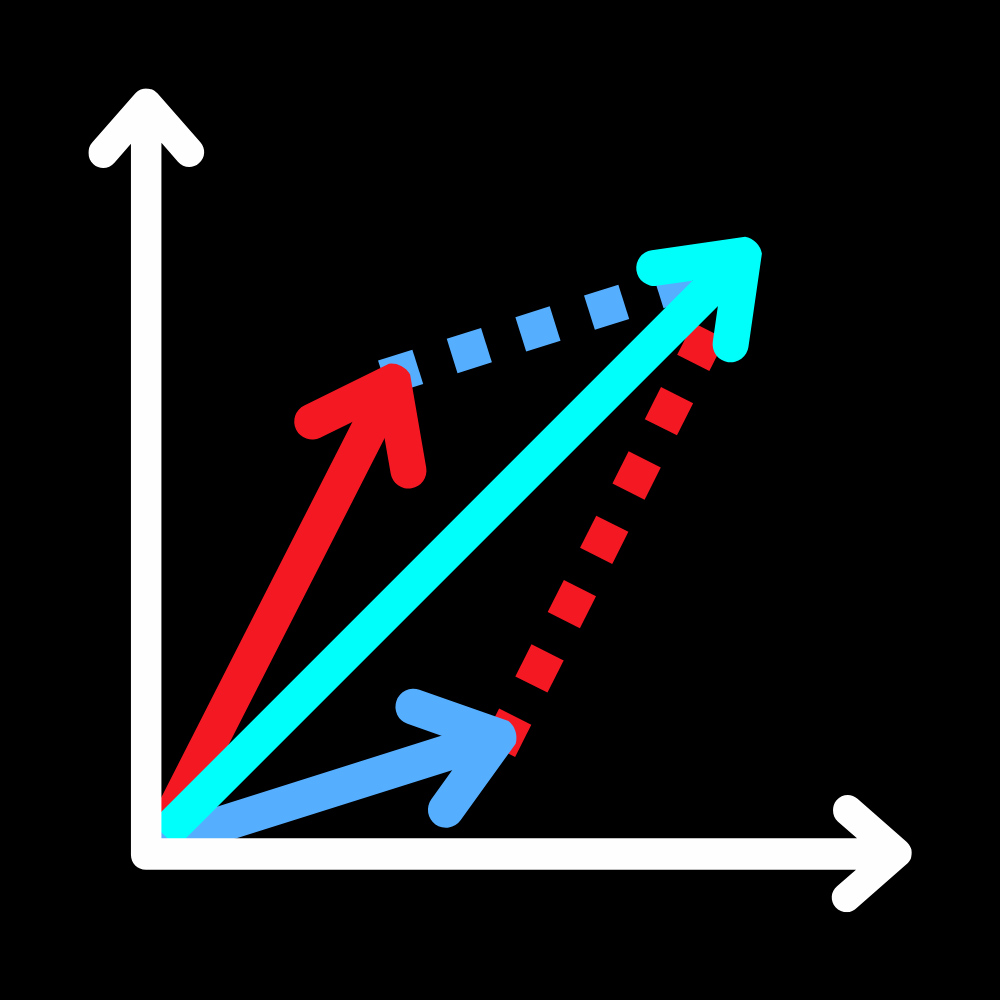

And that's it! That's pretty much all there is to basic vectors, since we aren't dealing with algebra and more advanced math. To close off the first lesson, we'll give you a little sneak preview of something about vectors.

Component Form

Vectors can be defined via something called components. In a 2-dimensional plane, we have a horizontal component (a horizontal vector with magnitude) and a vertical component (vertical vector with magnitude). The reason why we do this is because horizontal and vertical vectors are super easy to add (remember we said vectors in same direction can be added linearly?).

A vector in component form is typically addressed like so: $\vec{a} = \langle 1, 1 \rangle$, with the left number being the horizontal component and the vertical component. The reason why component form is so nice is because we can simply add and subtract the numbers in the funny brackets. For two vectors, $\vec{a}$ and $\vec{b}$, if $\vec{a} = \langle 4,5 \rangle$ and $\vec{n} = \langle 2,1 \rangle$, the resultant vector of $\vec{a} + \vec{b} = \langle 4+2,5+1 \rangle = \langle 6,6 \rangle$. If you want a diagram, see the one below: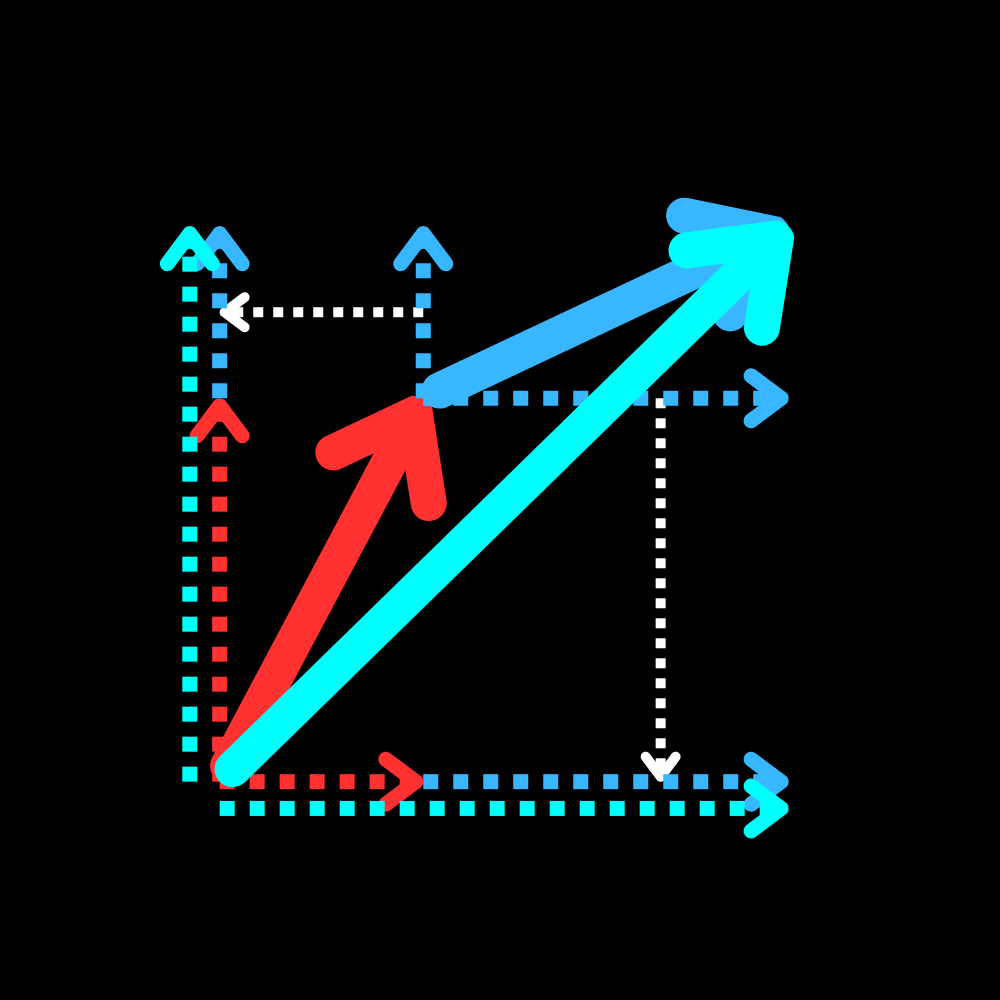

The diagram may be a little cluttered and difficult to understand, but you see the horizontal component of the RED vector plus the horizontal component of the BLUE vector is equal to the white vector's horizontal component (It's the three dashed vectors pointing to the right, close to the bottom of the diagram) and same goes for the vertical component.

The smaller, dashed white arrows show how you can move the BLUE vector's components to make the addition work, and since components are vectors, we can move them as long as we keep their magnitude and direction. This diagram just proves how you can simply add vector components, using what we just learned: the tip-to-tail method!

Conclusion

If you want to learn more about this, you can either search it up or take a sneak peek at our Algebra-based level (if you feel confident enough). Ready to go onto the next lesson? Let's hit it!

Algebraic Methods

This is great and all, but sometimes, graphical analysis is unavailable. In that case, algebraic vector addition is available. But it's not as simple as $1+1=2$! First, we will introduce the two methods of algebraically representing vectors. Being able to represent them algebraically is key for doing any sort of computation with them.

The first is to express a vector as a magnitude (length) and an angle, usually measured from the positive x-axis. The notation $|\vec{a}|$ represents the magnitude of vector $\vec{a}$. The angle $\theta$, or the argument of a vector, denoted as $\textrm{arg}(\vec{a}$), is the angle the vector makes with the positive x-axis. A figure is drawn below to show what we mean: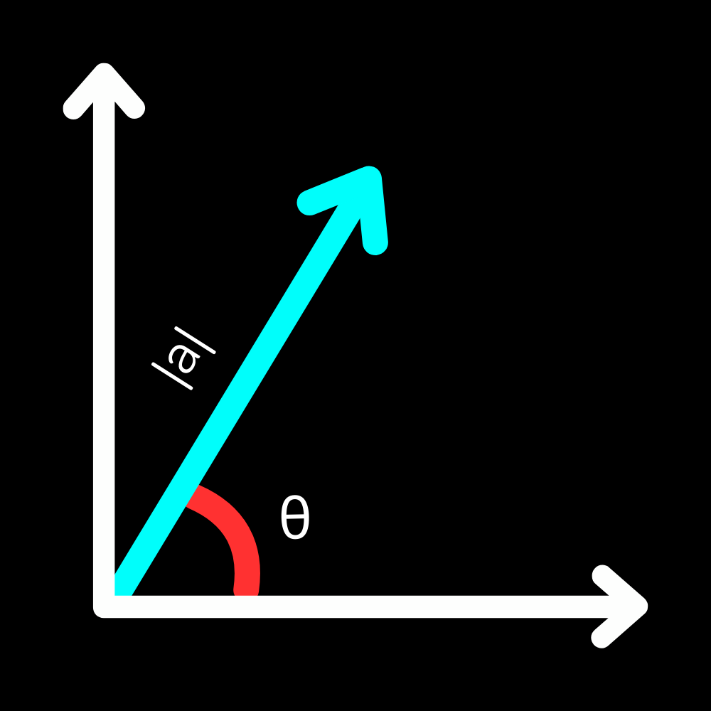

Component Form

The other method is to define a vector by its horizontal and vertical components. In this case, either angle brackets are used or the unit vector notation is used. The two are practically the same. In the angle bracket notation, a vector is represented by $\langle x,y \rangle$ where $x$ and $y$ are the lengths of the horizontal and vertical components of the vector, respectively.

IMPORTANT!! The horizontal component ALWAYS comes first when using the angle bracket notation!!

A negative value indicates the component is in the negative direction. If you actually consider the $x$ component as a horizontal vector, and the $y$ component as a vertical vector, they will sum up to the original vector.

The unit vector notation directly demonstrates this. A unit vector is a vector in a particular direction that has a magnitude of 1. The unit vector in the positive $x$ direction is represented by $\hat{i}$ and in the $y$ direction, $\hat{j}$. So, if we have a vector that can be written as $\langle 3,4 \rangle$, it can also be written as $3\hat{i}+4\hat{j}$. The $\hat{k}$ vector is also introduced in 3D, but we won’t worry about that. A diagram is provided below: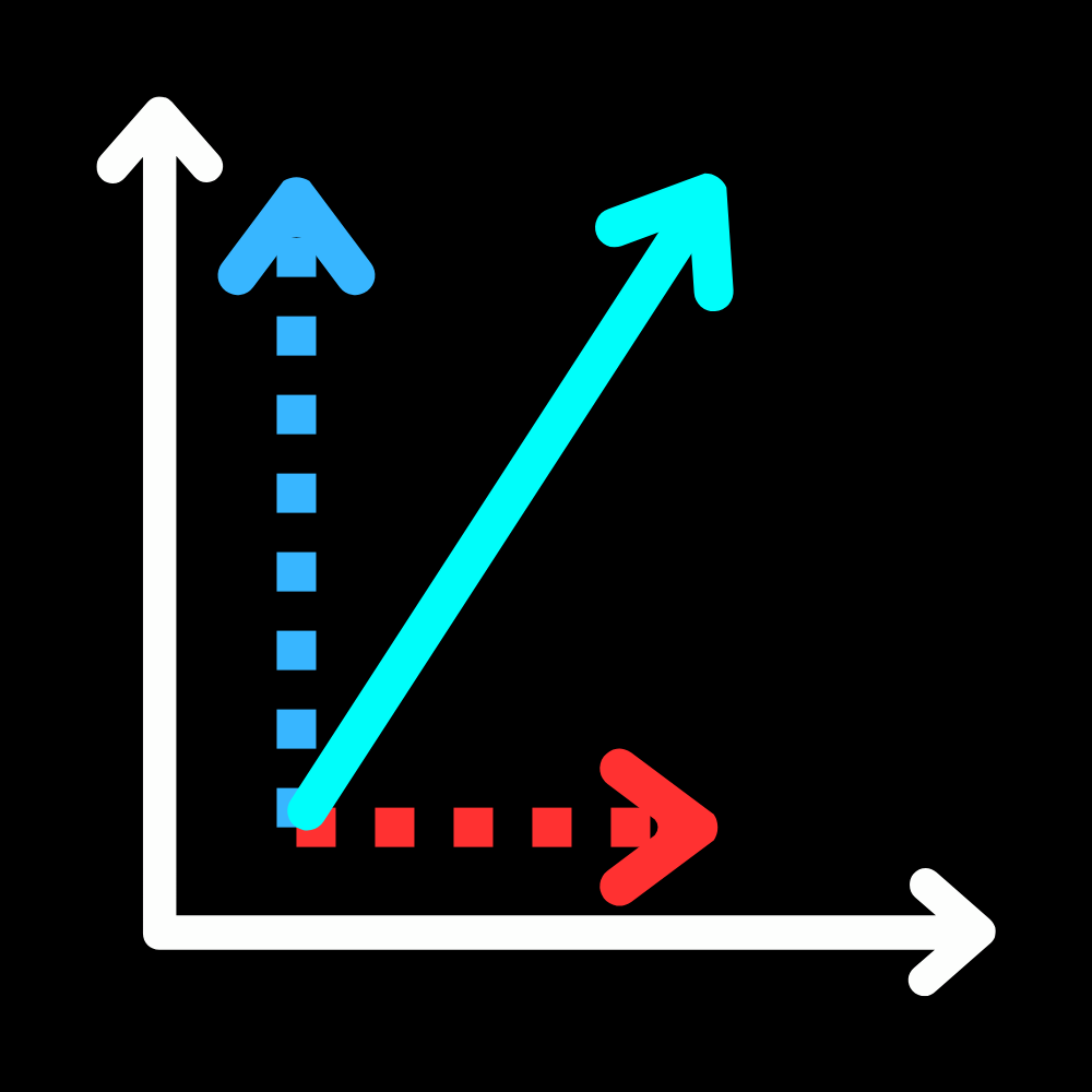

The method I will introduce here is the addition of vector components. NOTE: You can use the Law of Cosines as well, but we aren't covering that because it is more intensive on the calculation side and is not as useful in the context of vectors.

To add vectors algebraically, simply add their components. Yes, it is that simple! For instance, if $\vec{a} = \langle 3, 5 \rangle$ and $\vec{b} = \langle 4, 3 \rangle$ then $\vec{a} + \vec{b} = \langle 3+4,5+3 \rangle = \langle 7,8 \rangle$.

This, surprisingly, is actually nearly identical to graphically adding vectors, and here is a diagram as proof. I have excluded the coordinate axes to make the diagram less cluttered, but realize that we are still working in a coordinate plane:

Now is it clear that the components add up to the resultant vector? The red components add up with the blue components to produce the white components, as shown on the horizontal and vertical axes. The smaller, dashed white arrow shows you can move the components of the blue vectors to do tip-to-tail addition!

However, we may occasionally run into an issue here. How do we get the components of a vector if we are not given them? Suppose we are given the magnitude and argument (angle), as we mentioned before, instead. Well, the components of a vector are $\langle |\vec{a}|\cos(\theta),|\vec{a}|\sin(\theta) \rangle$ for vector $\vec{a}$ at an angle $\theta$ to the positive x-axis. This is due to basic right triangle trigonometry, and if you want to investigate more about this, you will have to do so on your own, since it would take too much effort to try to explain it here.

Conclusion

Whew! You made it to the end of the lesson on vectors! Congratulations! Physics is not an easy science to grasp, but you made it through the most basic and fundamental of all of it. The rest will be more concepts and less math (hopefully)! Ready to move on? Let's go!